| Name | Generates Tikz? | Export Options | Good For |
|---|---|---|---|
| ☆ q.uiver.app | Yes | HTML only | Commutative diagrams, graphs |
| mathcha.io | Yes | SVG, PDF, HTML | Geometrical drawings, plotting, all-purpose |
| Apple Keynote | No | SVG, PDF | Geometrical drawings, flowcharts |
During partial pivoting Guassian elimination (PPGE) of a matrix (just like regular GE, except we choose as a pivot the element which satisfies \({\max}_i|a_{ij}|\) for each column \(A^{(j)}\)), one sometimes accumulates large intermediate values——so much so that the final result in unreachable because of overflow. The following is a classical example: \[ A = \begin{bmatrix} 1 & 0 & 0 & 0 & 1\\ -1 & 1 & 0 & 0 & 1\\ -1 & -1 & 1 & 0 & 1\\ -1 & -1 & -1 & 1 & 1\\ -1 & -1 & -1 & -1 & 1\\ \end{bmatrix} \to \begin{bmatrix} 1 & 0 & 0 & 0 & 1\\ 0 & 1 & 0 & 0 & 2\\ 0 & 0 & 1 & 0 & 4\\ 0 & 0 & 0 & 1 & 8\\ 0 & 0 & 0 & 0 & 16\\ \end{bmatrix} = B \] For a \(n\) by \(n\) matrix as formulated above, PPGE will result in a matrices whose maximal element is \(2^{n-1}\). In fact, this is the worst case scenario. For much larger matrices, say $1000 \times 1000$, we are going to run into big problems. Despite this, PPGE is by far the most popular method for accomplishing LU decomposition and solving linear systems. Why? The catastrophic example above is possible, but probably won't happen.
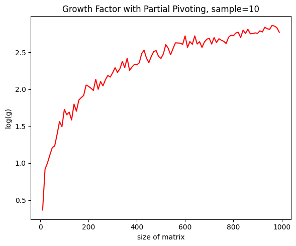
One calls the ratio of the maximal elements in absolute value of \(A\) and \(B\) the "growth factor" of \(A\), or \(g(A)\). As one would expect, the larger the matrix \(A\), the larger its growth factor (in the example above, this relationship is \(2^{n-1}\)):

This data is derived from normally distributed real matrices. Surprisingly, we don't see as exaggerated growth factors as the contrived example let on, and even the $\approx1000\times1000$ matrices are well suited for computation with PPGE. Hence: how likely is it that we run into examples remotely as bad as the initial example? We plot to find out that the answer is "almost never":

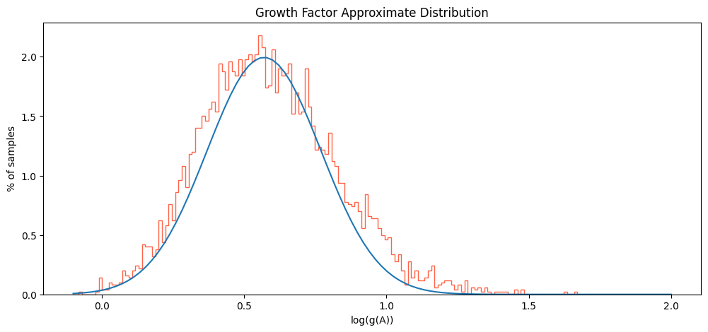
The above analysis only involves a few hundred sample matrices of each size. A sample of 5000 16x16 matrices yields similar behavior:

Which is to say, with growth factors that cap out at \(e^{1.7} \approx 5.5\), we are not ever getting close to the foretold bound of \(g(A) \leq 2^{16 }\approx 65,000\)
Completed as part of my evaluation for COMP 532, the following presentation gives a high-level overview of hard generators for propositional proof systems, their relevance to pseudorandomness, and a detailed width lower bound on Nisan-Wigderson generator hardness in resolution.

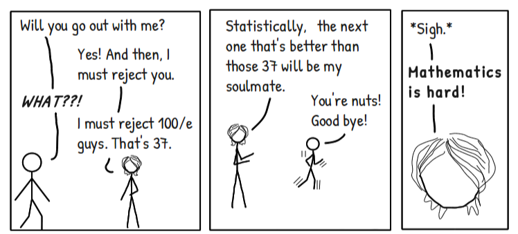
You are tying to find your soulmate, and thankfully \(N\) people have lined up for a "date." You don't know who exactly is the best candidate among them, but you can conduct interviews, one by one, to gather information. You can only interview a person once, and you must decide to choose them, or not, after the interview concludes. What strategy should you use to optimize the probability that, supposing your soulmate is in line, you pick him/her? The answer to this (preliminary) question is odd: you interview and reject \(k\) candidates, and then pick the first \((k+i)^{th}\) candidate who is better than all those previous. If \(k\) is picked ideally, the odds of choosing your soulmate are approximately \(1/e\), and what's more, the ideal ratio of \({k}/{N}\) is also \({1}/{e}\)! Here is the logic: \[ \begin{array}{rl} \mathbb{P}(\text{Soulmate chosen}) =& \; \mathbb{P}(\text{Soulmate chosen in \(k+1^{th}\) interview})\\ +& \; \mathbb{P}(\text{Soulmate chosen in \(k+2^{nd}\) interview})\\ \vdots&\\ +& \; \mathbb{P}(\text{Soulmate chosen in ${N}^{th}$ interview})\\ =& \sum_{i=1}^{N-k} \mathbb{P}(\text{Soulmate chosen in $(k+i)^{th}$ interview}) \end{array} \] Applying Bayes': \[\sum_{i=1}^{N-k}\mathbb{P}(S \text{ chosen @ } i) = \sum_{i=1}^{N-k}\mathbb{P}(\text{Given that }S_i = S, \; S_i \text{ chosen})\mathbb{P}(S_i = S)\] where \(S_i\) is the \(i^{th}\) person interviewed after the initial round of rejects, and \(S\) is your soulmate. Immediately, we see that the probability of any candidate being your soulmate, \(\mathbb{P}(S_i = S)\), is \({1}/{N}\). If \(S_i\) is given to be "the one," they are chosen only if the best candidate thus far was preliminarily rejected (otherwise, he/she would have been selected, not \(S_i\)). Thus, we have \(\mathbb{P}(S_i\text{ chosen | }S_i = S) = {k}/{(k+i-1)}\). \[\mathbb{P}(S \text{ is chosen}) = \sum_{i=1}^{N-k}\mathbb{P}(S \text{ chosen in interview } i) = \sum_{i=1}^{N-k}\frac{k}{N(k+i-1)}\] One can express this summation, using some calculus, as an approximation of a Riemann integral, as follows: \[m \int_{m}^{1}\frac{1}{x}dx = m\ln(x)\left|_{m}^{1}\right. = -m\ln(m)\] where \(m\) is the limiting case of \({k}/{N}\). When this expression is maximized by differentiating and setting to 0, one yields \({k}/{N} = {1}/{e} \), and thus the probability of picking your soulmate with the above-defined ratio is also \({1}/{e}\). That's 37%!
A Bézier curve interpolates between some data in \(\mathbb{R}^n\), usually points on a plane (one can shift control points to fit a desired shape, and it isn't too hard to succeed this way). Kaur and Goyal recently developed an "\(\alpha\)-Bézier," where, the larger the parameter \(\alpha \in \mathbb{R}\) is, the closer the Bézier interpolation will hug our control points. So, given some points in \(\mathbb{R}^2\), we could observe increasingly strict interpolations.
What we have above is an interpolation of some points, parameterized over how "tight" the interpolation is. It's like math shrinkwrap!
A Bézier curve typically maps the unit interval onto a curve in \(\mathbb{R}^n\). One can generate a "curve of curves" to map the unit square onto a surface. This is called a tensor product surface, or Bézier surface, in the case of ordinary Bézier curves. The math: \[ \{ T(t, s) \}_{\alpha \in (-1, 3)} = \left\{\sum{_{i=0}^{3}}\sum{_{j=0}^{3}}B_i^n(t, \alpha)B_j^m(s, \alpha)\vec{v_{ij}} : \alpha \in (-1, 3) \right\} \leftarrow \text{ tensor surface computation}\] \[\text{where } B_i^n := \left[\binom{n-2}{i}(1-\alpha)t + \binom{n-2}{i-2}(1-\alpha)(1-t) +\binom{n}{i} \alpha t(1-t)\right]t^{i-1}(1-t)^{n-i-1} \leftarrow \text{ alpha-Bezier}\]